Just as weather forecasting is valuable in our daily lives, time-series forecasting plays an important role in business decisions. Today, massive data is gathered through automations and systems every day, making time-series data increasingly prevalent and accessible. Consequently, the ability to learn from these time-series data and generate accurate forecasts for the future is becoming ever more essential.
In business, forecasting is not only about the numbers but also about setting expectations for the future and allocating resources ahead of the change that is expected to happen. Good forecasting influences various aspects of business operations and decisions, including inventory management, performance evaluation, and employee scheduling. Not only optimization of resources, but also good forecasting can enhance company collaboration. It aligns goals across the departments with transparency, encourages proactive strategies rather than reactive strategies, and fosters a culture of trust where teams feel more connected to the company’s objectives and to each other.
This is where machine learning and data science play a critical role. Most modern machine learning frameworks didn’t originate from time-series problems, but when people experiment with those models into time-series data, they found good results. People have managed to use techniques like lag and time-series split to make the models able to learn the trend and seasonality inside time-series data, and yield decent forecasting results.
In this post, we are going to talk about the problem I’ve encountered when forecasting business metrics using machine learning models, how I choose models and why, the lag and cross-validation techniques to use, and how to interpret model results to business users.
Problems for real-world time series data:
Seasonal nature
Business data often show seasonalities. To capture this kind of information, date components (calendar features) are often used as input to the forecasting, such as month, day of the month, and day of the week.
A lag of the appropriate length also helps in forecasting seasonalities. For example, when the data is monthly, a lag length of 12 means that the target value from the same period of the previous year is used in forecasting the target.
Let’s say you want to forecast the value of T at time 101 T_{101}. Lag is creating columns by shifting the values of a particular feature back by a certain number of time periods. These lagged columns are then used as independent variables in conjunction with the existing row values.
Lag of Length 1:
Use the value of T at time 100 T_{100} for this forecast. Since T_{100} is the immediate predecessor of T_{101}, this is a lag of length 1.
Lag of Length 2:
Or, we use the value from time 99 T_{99}. Since there is one intervening time point T_{100} between T_{99} and T_{101}, this constitutes a lag of length 2.
Multivariate nature
Say you have target T, the time series you want to predict. You also have feature E, the exogenous variable you want to incorporate. Then you can create lags, T_{t-2}, T_{t-1}, T_{t} in order to predict T_{t+1}, you can also add lags for exogenous variables E_{t-2}, E_{t-1}, E_{t} and add them to your rows.
In real-world business settings, data is typically collected from multiple systems or through data integrations and possesses a richness of features to be used in the forecasting model. When building a time series forecasting model in business, it always incorporates multiple variables (along with their respective histories) as inputs to predict future metrics.
This richness in dimensions can lead to a problem known as the curse of dimensionality, especially harmful for time series forecasting because time-series feature engineering often involves transforming one feature into multiple features to capture changes over time.
Based on my own experience and observations from numerous Kaggle competition first-place solutions, it is typically necessary to calculate certain features in order to generate an accurate forecast. These features include:
- Lags
- Moving averages
- Moving standard deviations
- Features based on the target
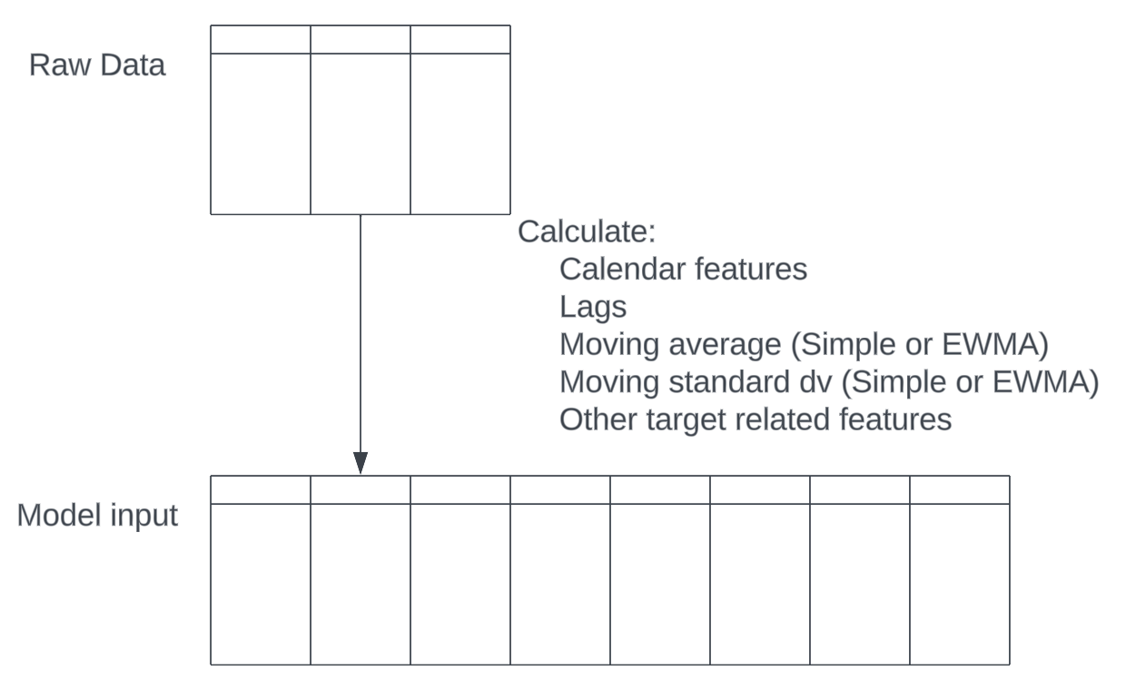
This essentially increases the input dimensionality by 4–5 times, and creating lag features will multiply the dimensionality again! A usually selected lag length is 6–12. Considering all of this, the real input dimensionality can reach 20+ times the raw data dimensionality, which will cause the curse of dimensionality. Training machine learning models with too many features but limited rows is like finding a needle in a haystack: the computation will be heavy, and overfitting is risky.
Need for Interpretability
Interpreting the model output has been a tier-1 problem for time-series forecasting in businesses. Especially when the forecast deviates, business users need to understand what is happening and why. This is crucial for building trust with business users. When people can understand the model to some extent and know where the forecasting comes from, they can trust it more and use it more effectively for decision-making. That’s why so many companies are still content with linear forecasting: People understand the parameters of linear models and know when to trust the forecast, using it as a benchmark for making decisions. On the contrary, most neural networks have terrible Interpretability, and people are always skeptical about these kinds of black boxes.
Model Selection: Tree-based model like GBM
Before diving too deep and trying to train a model with the least cv MSE, think about the problem and goal first. If the goal is to provide a benchmark for your sales team to set the quarterly goal, maybe a simple linear model will be the best choice. However, if the goal is to help the supply-chain department forecast demand for inventory management. Then accuracy and seasonality is the critical part. Sometimes a single model isn’t enough, you’ll probably use bagging to ensemble multiple model results, or stack a model to a well-established model to predict the residual.
Nevertheless, Tree-based models like Random Forests and Gradient Boosting Machines (GBM) stand out in fulfilling several key needs in time series forecasting. They are capable of dealing with multivariate data and high dimensionality. They provide good accuracy as well as interpretability.
Adept at coping with multivariate data and high dimensionality
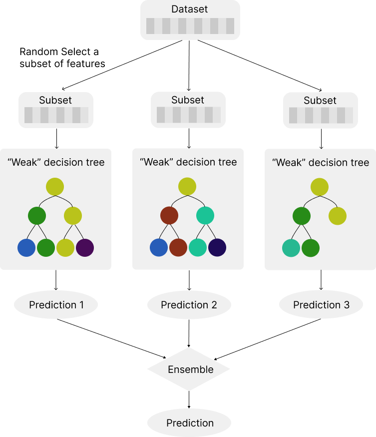
Tree-based models can capture complex, non-linear relationships between features and the lag features. For random forests and Boosting machines, the model is assembled by many individual trees. Each individual tree acts as a “weak” predictor, which is intentionally limited in complexity. Instead of using all the features of your problem, individual trees work with only a subset of the features and control the tree depth. This minimizes the solution space that each tree is optimizing over and can help combat the problem of the curse of dimensionality. On its own, a single tree might not perform very well or might be overly simplistic. However, when combined with many others in the boosting process, these weak learners collectively form a strong predictive model that performs well with high dimensionality.
Accuracy
Tree-based models like LightGBM are still the top-tier accuracy models when it comes to multivariate time series forecasting. Even for the first-place solutions in recent Kaggle competitions, tree-based models are one of the ensemble components of the solution. This comes from the ability of tree-based models to capture the trend, repeat patterns, and remove noise. But you need to do some proper feature engineering according to the data. The lag and moving average columns we mentioned above are absolutely critical, and there are also some other techniques to better capture seasonality and trend, see Kaggle grandmaster’s blog: https://towardsdatascience.com/better-features-for-a-tree-based-model-d3b21247cdf2
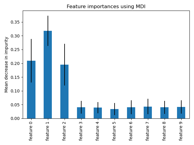
Descent interpretability:
Despite being more complex than linear models, tree-based models like Random Forests and Gradient Boosting Machines (GBM) offer decent interpretability because they provide a feature importance score for all the features. This is because in each step of building the trees, the model selects the feature that best splits the data, often based on criteria such as Gini impurity or information gain. Gini impurity measures how often a randomly chosen element would be incorrectly labeled if it was randomly labeled according to the distribution of labels in the subset. The reduction in this impurity over all the trees in the forest is used to compute the Feature Importance Scores for each feature, indicating how much each feature contributes to the decision-making process of the model. This can help in understanding which features are contributing most to the predictions.
This brings insight to analytics. People can understand which variables (like weather, in your example) most strongly influence the target variable (like sales), and more importantly, it builds trust with business users. For instance, if weather is a top feature affecting sales, and this aligns with business users’ experience or intuition, it reinforces the model’s credibility. Sometimes, feature importance can reveal unexpected predictors, which might not have been considered significant in traditional analyses. These insights can actually open up new avenues for business strategy or prompt further investigation into why these features are impactful. Analyzing, and more importantly communicating feature importance with stakeholders, bridge the gap between complex machine learning models and business users.
Other models:
Many deep-learning based models have also gained popularity in time series analysis, thanks to architectures like Temporal Convolutional Network, LSTM, and Transformer, which have achieved impressive results on some datasets.
However, a significant drawback of these DNN models is their ‘black box’ nature, making it extremely challenging for business users to interpret the results. Furthermore, their performance is not consistently superior across all datasets. In some cases, a simple exponential smoothing model may outperform these complex, computationally intensive models (Kaggle M5 paper). Even for solutions that employ deep-learning-based models, they typically use these as a base model and combine them with tree-based models and other types of models.
Given the lack of visibility into how the model functions, and the occasional occurrence of poor results, how can it gain the trust of business users and influence business decisions? This situation makes it challenging to use deep-learning based models in business settings.
Conclusion:
The richness of time series data and the demand for both accurate and explainable models for forecasting in business scenarios lead to a preference for tree-based models like Random Forest, XGboost, and lightGBM. These models typically perform well in terms of accuracy, are less prone to overfitting, thus demonstrating good generalizability to new datasets, and provide visibility and interpretability through feature importance scores.
Still, tree-based models have their own limitations, such as it sucks at long-term forecasting. The selection of an optimal model for a specific problem ultimately requires practical application and experimentation.
Do you agree with me? Feel free to leave your opinion as a comment!